40 add data labels to excel chart
Adding Data Labels to Your Chart - Excel ribbon tips 27 Aug 2022 — Activate the chart by clicking on it, if necessary. · Make sure the Layout tab of the ribbon is displayed. · Click the Data Labels tool. Excel ... How to create Custom Data Labels in Excel Charts - Efficiency 365 Two ways to do it. Click on the Plus sign next to the chart and choose the Data Labels option. We do NOT want the data to be shown. To customize it, click on the arrow next to Data Labels and choose More Options … Unselect the Value option and select the Value from Cells option. Choose the third column (without the heading) as the range.
How to Add Total Data Labels to the Excel Stacked Bar Chart Step 4: Right click your new line chart and select "Add Data Labels" Step 5: Right click your new data labels and format them so that their label position is "Above"; also make the labels bold and increase the font size. Step 6: Right click the line, select "Format Data Series"; in the Line Color menu, select "No line" Step 7 ...
Add data labels to excel chart
How to Add Data Labels to Scatter Plot in Excel (2 Easy Ways) - ExcelDemy Follow the ways we stated below to remove data labels from a Scatter Plot. 1. Using Add Chart Element At first, go to the sheet Chart Elements. Then, select the Scatter Plot already inserted. After that, go to the Chart Design tab. Later, select Add Chart Element > Data Labels > None. This is how we can remove the data labels. How to add text labels on Excel scatter chart axis - Data Cornering Here is the data that I would like to display in the Excel scatter chart. In addition, I would like to add custom labels on Excel scatter chart x-axis with each person's name. Stepps to add text labels on Excel scatter chart axis. 1. Firstly it is not straightforward. Excel scatter chart does not group data by text. How To Create Labels In Excel - npvltd.info A dialog box called a new name is. In this second method, we will add the x and y axis labels in excel by chart element button. 4 quick steps to add two data labels in excel chart. Go To Mailing Tab > Select. Click yes to merge labels from excel to word. Under select document type choose labels. click next. the label options box will open.
Add data labels to excel chart. How to Use Cell Values for Excel Chart Labels - How-To Geek Select the chart, choose the "Chart Elements" option, click the "Data Labels" arrow, and then "More Options." Uncheck the "Value" box and check the "Value From Cells" box. Select cells C2:C6 to use for the data label range and then click the "OK" button. The values from these cells are now used for the chart data labels. Data Labels in Excel Pivot Chart (Detailed Analysis) Before adding the Data Labels, we need to create the Pivot Chart in the beginning. We can create a Pivot Chart from the Insert tab. To do this, go to Insert tab > Tables group. Then in the dialog box, select the range of cells of the primary dataset., here the range of cells is B4:J23. And select the New Worksheet in the next option. How to Add Labels to Scatterplot Points in Excel - Statology Step 3: Add Labels to Points. Next, click anywhere on the chart until a green plus (+) sign appears in the top right corner. Then click Data Labels, then click More Options…. In the Format Data Labels window that appears on the right of the screen, uncheck the box next to Y Value and check the box next to Value From Cells. How to Add Two Data Labels In Excel Chart? - YouTube In this video tutorial, we are going to learn, how to add multiple data labels in excel pie chart.Our YouTube Channels Travel Volg Channelhttps:// ...
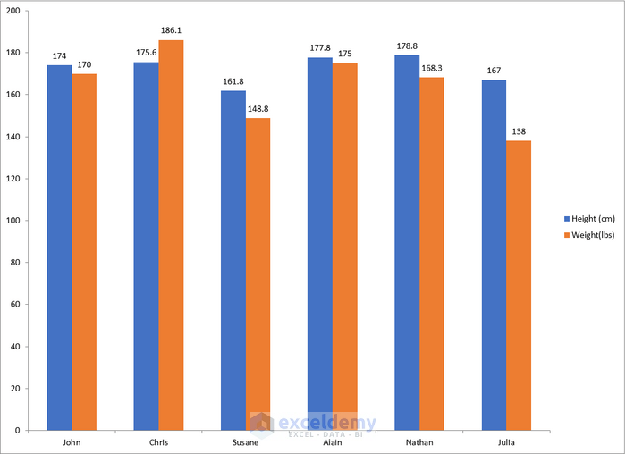
Edit titles or data labels in a chart - support.microsoft.com On a chart, click one time or two times on the data label that you want to link to a corresponding worksheet cell. The first click selects the data labels for the whole data series, and the second click selects the individual data label. Right-click the data label, and then click Format Data Label or Format Data Labels. How to Add Two Data Labels in Excel Chart (with Easy Steps) Table of Contents hide. Download Practice Workbook. 4 Quick Steps to Add Two Data Labels in Excel Chart. Step 1: Create a Chart to Represent Data. Step 2: Add 1st Data Label in Excel Chart. Step 3: Apply 2nd Data Label in Excel Chart. Step 4: Format Data Labels to Show Two Data Labels. Things to Remember. How to add data labels from different columns in an Excel chart? 10 Sept 2022 — To add data labels, right-click the set of data in the chart, then pick the Add Data Labels option in Add Data Labels from the context menu. How To Add Data Labels In Excel - computerinnovations.info To do this, click the "format" tab within the "chart tools" contextual tab in the ribbon. Use the following steps to add data labels to series in a chart: Source: pakaccountants.com. Add custom data labels from the column "x axis labels". In this second method, we will add the x and y axis labels in excel by chart element button.
Adding Data Labels To An Excel Chart | MyExcelOnline In our example below, I add a Data Label to a column chart and then I format the data label using CTRL+1. I then select to custom format the numbers so it shows the values as thousands by adding a comma , after each zero and then showing the work k by adding "k" Example Custom Number Format: [$$-1004]#,##0 ,"k" ;- [$$-1004]#,##0 ,"k" How To Add Data Labels In Excel - numeros-emergencia.info Click add chart element chart elements button > data labels in the upper. Next Open Format Data Labels By Pressing The More Options In The Data Labels. Make row labels in excel 2007 freeze for easier reading from . 47 rows add a label (form control) click developer, click insert, and then click label. This is the key step! Add a DATA LABEL to ONE POINT on a chart in Excel Click on the chart line to add the data point to. All the data points will be highlighted. Click again on the single point that you want to add a data label to. Right-click and select ' Add data label ' This is the key step! Right-click again on the data point itself (not the label) and select ' Format data label '. How to add data labels in excel to graph or chart (Step-by-Step) Add data labels to a chart. 1. Select a data series or a graph. After picking the series, click the data point you want to label. 2. Click Add Chart Element Chart Elements button > Data Labels in the upper right corner, close to the chart. 3. Click the arrow and select an option to modify the location. 4.
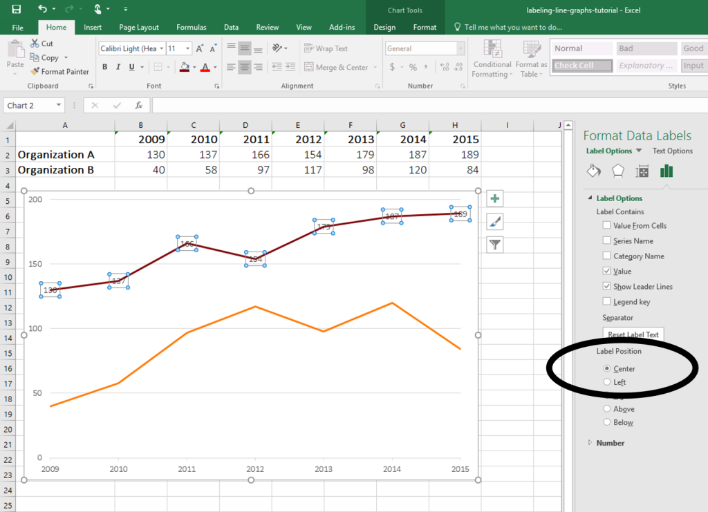
How to Place Labels Directly Through Your Line Graph in ...
Add data labels to your Excel bubble charts | TechRepublic Right-click the data series and select Add Data Labels. Right-click one of the labels and select Format Data Labels. Select Y Value and Center. Move any labels that overlap. Select...
Add Data Labels Outside End for Dynamic Label Threshold Chart ...
How to add or move data labels in Excel chart? - ExtendOffice To add or move data labels in a chart, you can do as below steps: In Excel 2013 or 2016. 1. Click the chart to show the Chart Elements button .. 2. Then click the Chart Elements, and check Data Labels, then you can click the arrow to choose an option about the data labels in the sub menu.See screenshot:

How to add data labels from different column in an Excel chart?
Find, label and highlight a certain data point in Excel scatter graph Here's how: Click on the highlighted data point to select it. Click the Chart Elements button. Select the Data Labels box and choose where to position the label. By default, Excel shows one numeric value for the label, y value in our case. To display both x and y values, right-click the label, click Format Data Labels…, select the X Value and ...

Add Data Labels for Total to Stacked Columns in #Excel | wmfexcel
Create Dynamic Chart Data Labels with Slicers - Excel Campus This is because Excel 2010 does not contain the Value from Cells feature. Jon Peltier has a great article with some workarounds for applying custom data labels. This includes using the XY Chart Labeler Add-in, which is a free download for Windows or Mac. Step 6: Setup the Pivot Table and Slicer. The final step is to make the data labels ...

424 How to add data label to line chart in Excel 2016
Add data labels and callouts to charts in Excel 365 The steps that I will share in this guide apply to Excel 2021 / 2019 / 2016. Step #1: After generating the chart in Excel, right-click anywhere within the chart and select Add labels . Note that you can also select the very handy option of Adding data Callouts.
/simplexct/BlogPic-idc97.png)
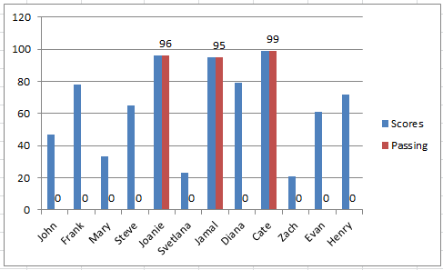
How to Create a Bar Chart With Labels Inside Bars in Excel
Add or remove data labels in a chart - support.microsoft.com Add data labels to a chart Click the data series or chart. To label one data point, after clicking the series, click that data point. In the upper right corner, next to the chart, click Add Chart Element > Data Labels. To change the location, click the arrow, and choose an option.

Add data labels and callouts to charts in Excel 365 ...
How to Add Data Labels in Excel - Excelchat | Excelchat After inserting a chart in Excel 2010 and earlier versions we need to do the followings to add data labels to the chart; Click inside the chart area to display the Chart Tools. Figure 2. Chart Tools Click on Layout tab of the Chart Tools. In Labels group, click on Data Labels and select the position to add labels to the chart. Figure 3.

Microsoft Excel Tutorials: Add Data Labels to a Pie Chart
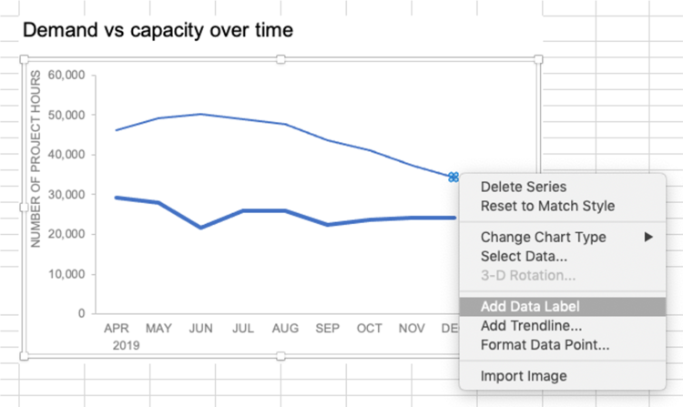
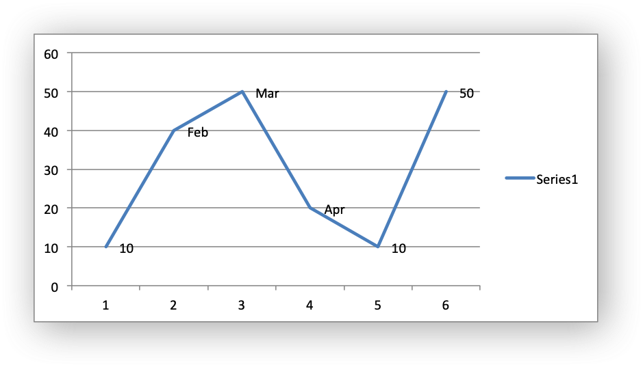
how to add data labels into Excel graphs You can download the corresponding Excel file to follow along with these steps: Right-click on a point and choose Add Data Label. You can choose any point to add a label—I'm strategically choosing the endpoint because that's where a label would best align with my design. Excel defaults to labeling the numeric value, as shown below.

Excel Charts: Dynamic Label positioning of line series
How to Add Data Labels to an Excel 2010 Chart - dummies On the Chart Tools Layout tab, click Data Labels→More Data Label Options. The Format Data Labels dialog box appears. You can use the options on the Label Options, Number, Fill, Border Color, Border Styles, Shadow, Glow and Soft Edges, 3-D Format, and Alignment tabs to customize the appearance and position of the data labels.
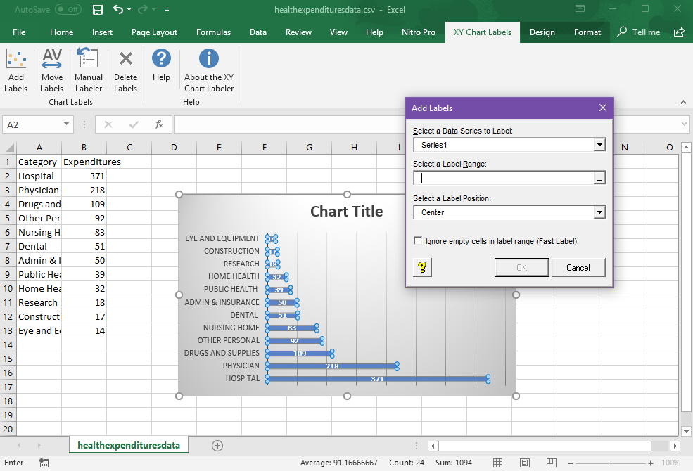
Add Labels to XY Chart Data Points in Excel with XY Chart Labeler
How to add data labels from different column in an Excel chart? Right click the data series in the chart, and select Add Data Labels > Add Data Labels from the context menu to add data labels. 2. Click any data label to select all data labels, and then click the specified data label to select it only in the chart. 3.
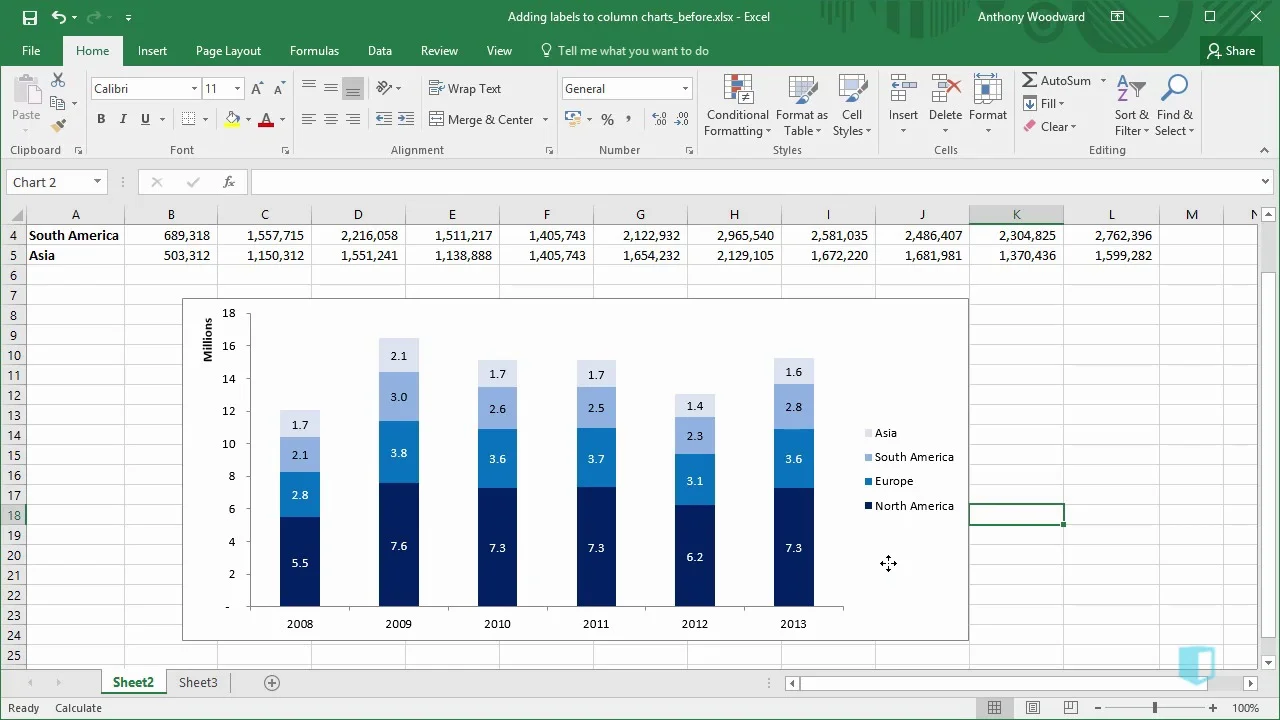
Adding Labels to Column Charts | Online Excel - KPMG Tax - Digital Now Course Training
Change the format of data labels in a chart To get there, after adding your data labels, select the data label to format, and then click Chart Elements > Data Labels > More Options. To go to the appropriate area, click one of the four icons ( Fill & Line, Effects, Size & Properties ( Layout & Properties in Outlook or Word), or Label Options) shown here.

How to add live total labels to graphs and charts in Excel ...
Custom Chart Data Labels In Excel With Formulas - How To Excel At Excel Follow the steps below to create the custom data labels. Select the chart label you want to change. In the formula-bar hit = (equals), select the cell reference containing your chart label's data. In this case, the first label is in cell E2. Finally, repeat for all your chart laebls.

microsoft excel - Adding data label only to the last value ...
How To Create Labels In Excel - npvltd.info A dialog box called a new name is. In this second method, we will add the x and y axis labels in excel by chart element button. 4 quick steps to add two data labels in excel chart. Go To Mailing Tab > Select. Click yes to merge labels from excel to word. Under select document type choose labels. click next. the label options box will open.

How-to Use Data Labels from a Range in an Excel Chart - Excel ...
How to add text labels on Excel scatter chart axis - Data Cornering Here is the data that I would like to display in the Excel scatter chart. In addition, I would like to add custom labels on Excel scatter chart x-axis with each person's name. Stepps to add text labels on Excel scatter chart axis. 1. Firstly it is not straightforward. Excel scatter chart does not group data by text.

Apply Custom Data Labels to Charted Points - Peltier Tech
How to Add Data Labels to Scatter Plot in Excel (2 Easy Ways) - ExcelDemy Follow the ways we stated below to remove data labels from a Scatter Plot. 1. Using Add Chart Element At first, go to the sheet Chart Elements. Then, select the Scatter Plot already inserted. After that, go to the Chart Design tab. Later, select Add Chart Element > Data Labels > None. This is how we can remove the data labels.

Enable or Disable Excel Data Labels at the click of a button ...

Chart Data Labels in PowerPoint 2011 for Mac

How to Add Data Labels in Excel - Excelchat | Excelchat

Custom Data Labels with Colors and Symbols in Excel Charts ...

Add or remove data labels in a chart

How to Add Total Data Labels to the Excel Stacked Bar Chart ...
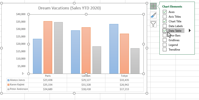
How to Add Data Tables to a Chart in Excel - Business ...
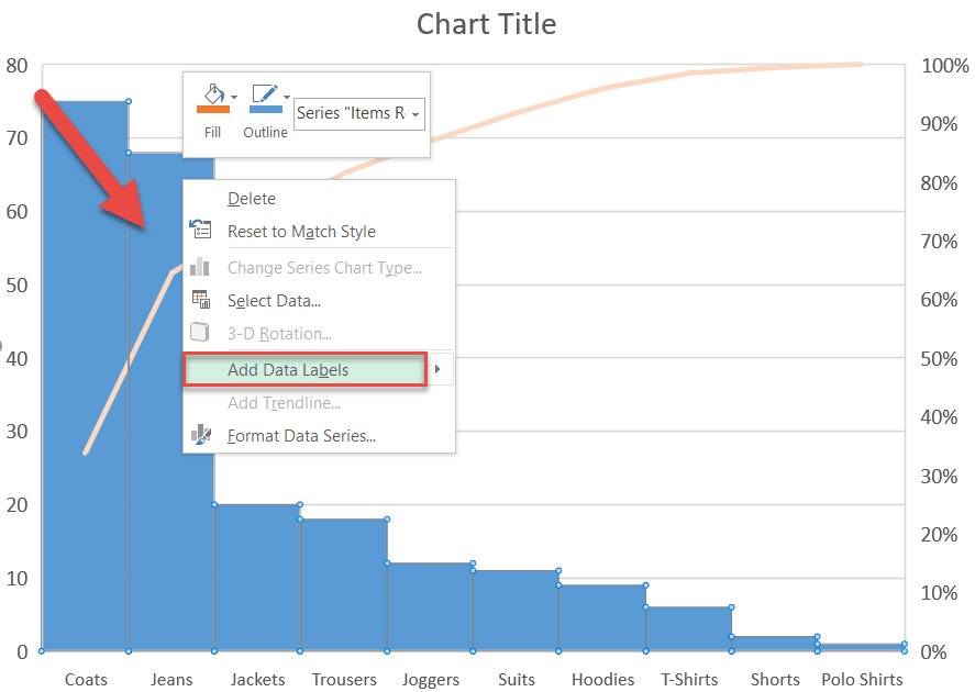
How to Create a Pareto Chart in Excel – Automate Excel

Add or remove data labels in a chart

How to Add Axis Labels to a Chart in Excel | CustomGuide

Change the format of data labels in a chart
how to add data labels into Excel graphs — storytelling with data

microsoft excel - Adding data label only to the last value ...

Directly Labeling Excel Charts - PolicyViz

How to Add Data Labels to an Excel 2010 Chart - dummies

Custom data labels in a chart

How to Customize Your Excel Pivot Chart Data Labels - dummies

How to Add Total Data Labels to the Excel Stacked Bar Chart ...
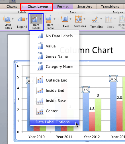
Format Data Label Options in PowerPoint 2011 for Mac
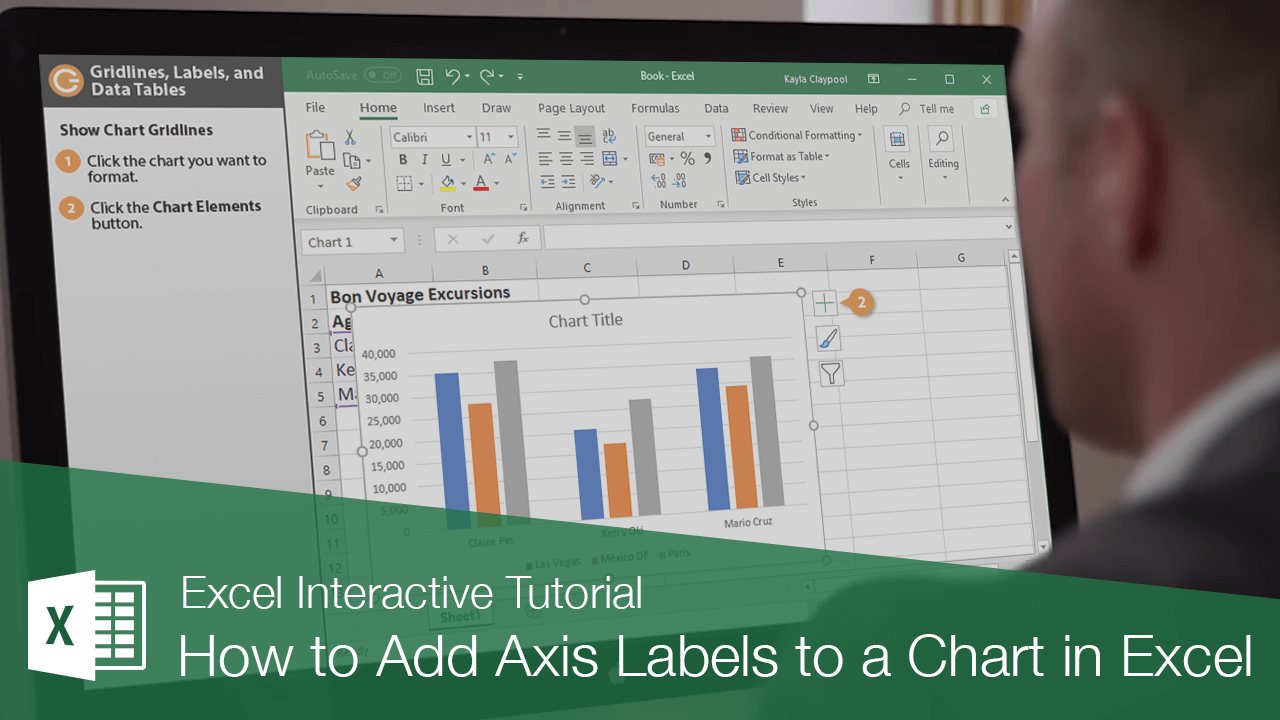
How to Add Axis Labels to a Chart in Excel | CustomGuide

Format Data Labels in Excel- Instructions - TeachUcomp, Inc.

Change the format of data labels in a chart
How to Add Data Labels in Excel (2 Handy Ways) - ExcelDemy
Working with Charts — XlsxWriter Documentation

How to add data labels from different column in an Excel chart?
Post a Comment for "40 add data labels to excel chart"