41 excel chart add data labels
Adding Data Labels to Your Chart (Microsoft Excel) To add data labels, follow these steps: Activate the chart by clicking on it, if necessary. Choose Chart Options from the Chart menu. Excel displays the Chart Options dialog box. Make sure the Data Labels tab is selected. (See Figure 1.) The left side of the dialog box shows the different types of data labels you can choose. Adding Data Labels to Your Chart (Microsoft Excel) To add data labels in Excel 2013 or Excel 2016, follow these steps: Activate the chart by clicking on it, if necessary. Make sure the Design tab of the ribbon is displayed. (This will appear when the chart is selected.) Click the Add Chart Element drop-down list. Select the Data Labels tool.
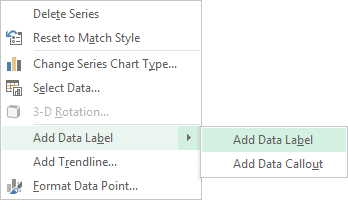
Add a DATA LABEL to ONE POINT on a chart in Excel Click on the chart line to add the data point to. All the data points will be highlighted. Click again on the single point that you want to add a data label to. Right-click and select 'Add data label' This is the key step! Right-click again on the data point itself (not the label) and select 'Format data label'.

Excel chart add data labels
Chart.ApplyDataLabels method (Excel) | Microsoft Docs The type of data label to apply. True to show the legend key next to the point. The default value is False. True if the object automatically generates appropriate text based on content. For the Chart and Series objects, True if the series has leader lines. Pass a Boolean value to enable or disable the series name for the data label. How to add data labels from different column in an Excel chart? Please do as follows: 1. Right click the data series in the chart, and select Add Data Labels > Add Data Labels from the context menu to add... 2. Right click the data series, and select Format Data Labels from the context menu. 3. In the Format Data Labels pane, under Label Options tab, check the ... Adding Data Labels To An Excel Chart | MyExcelOnline In our example below, I add a Data Label to a column chart and then I format the data label using CTRL+1. I then select to custom format the numbers so it shows the values as thousands by adding a comma , after each zero and then showing the work k by adding "k" Example Custom Number Format: [$$-1004]#,##0 ,"k" ;- [$$-1004]#,##0 ,"k"
Excel chart add data labels. Add or remove data labels in a chart - support.microsoft.com Add data labels to a chart Click the data series or chart. To label one data point, after clicking the series, click that data point. In the upper right corner, next to the chart, click Add Chart Element > Data Labels. To change the location, click the arrow, and choose an option. If you want to ... How to Add Labels to Scatterplot Points in Excel - Statology Next, click anywhere on the chart until a green plus (+) sign appears in the top right corner. Then click Data Labels, then click More Options… In the Format Data Labels window that appears on the right of the screen, uncheck the box next to Y Value and check the box next to Value From Cells. how to add data labels into Excel graphs - storytelling with data You can download the corresponding Excel file to follow along with these steps: Right-click on a point and choose Add Data Label. You can choose any point to add a label—I'm strategically choosing the endpoint because that's where a label would best align with my design. Excel defaults to labeling the numeric value, as shown below. Multiple Data Labels on bar chart? - Excel Help Forum Add label to the second serie, outside of the bar Edit separately each label, egal to % value with formula to be dynamic Set the overlap to 100% Insert title with formula Hope this helps Best regards Attached Files sample chart two data labels_jpr73.xlsx (12.1 KB, 1251 views) Download Register To Reply 01-26-2012, 11:11 AM #6 Andy Pope Forum Guru
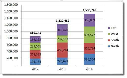
How to Make a Pie Chart in Excel & Add Rich Data Labels to The Chart! Creating and formatting the Pie Chart. 1) Select the data. 2) Go to Insert> Charts> click on the drop-down arrow next to Pie Chart and under 2-D Pie, select the Pie Chart, shown below. 3) Chang the chart title to Breakdown of Errors Made During the Match, by clicking on it and typing the new title. Custom Chart Data Labels In Excel With Formulas Follow the steps below to create the custom data labels. Select the chart label you want to change. In the formula-bar hit = (equals), select the cell reference containing your chart label's data. In this case, the first label is in cell E2. Finally, repeat for all your chart laebls. How to Use Cell Values for Excel Chart Labels Select the chart, choose the "Chart Elements" option, click the "Data Labels" arrow, and then "More Options." Uncheck the "Value" box and check the "Value From Cells" box. Select cells C2:C6 to use for the data label range and then click the "OK" button. The values from these cells are now used for the chart data labels. How to Add Total Data Labels to the Excel Stacked Bar Chart The basic chart function does not allow you to add a total data label that accounts for the sum of the individual components. Fortunately, creating these labels manually is a fairly simply process. Step 1: Create a sum of your stacked components and add it as an additional data series (this will distort your graph initially)
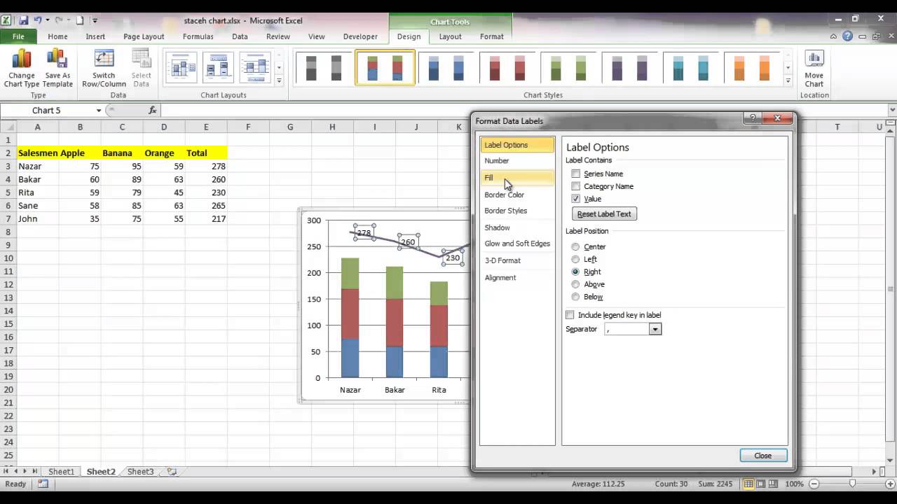
Add data labels and callouts to charts in Excel 365 | EasyTweaks.com Step #1: After generating the chart in Excel, right-click anywhere within the chart and select Add labels . Note that you can also select the very handy option of Adding data Callouts. Edit titles or data labels in a chart - support.microsoft.com On a chart, click one time or two times on the data label that you want to link to a corresponding worksheet cell. The first click selects the data labels for the whole data series, and the second click selects the individual data label. Right-click the data label, and then click Format Data Label or Format Data Labels. Apply Custom Data Labels to Charted Points - Peltier Tech With a chart selected, click the Add Labels ribbon button (if a chart is not selected, a dialog pops up with a list of charts on the active worksheet). A dialog pops up so you can choose which series to label, select a worksheet range with the custom data labels, and pick a position for the labels. How to Add Data Labels to an Excel 2010 Chart - dummies Select where you want the data label to be placed. Data labels added to a chart with a placement of Outside End. On the Chart Tools Layout tab, click Data Labels→More Data Label Options. The Format Data Labels dialog box appears.
E-xcel Tuts: Add Data Labels to Excel Charts
Add data labels to your Excel bubble charts | TechRepublic Right-click the data series and select Add Data Labels. Right-click one of the labels and select Format Data Labels. Select Y Value and Center. Move any labels that overlap. Select the data labels ...
Creating a chart with dynamic labels - Microsoft Excel 2013
Add / Move Data Labels in Charts - Excel & Google Sheets Adding Data Labels Click on the graph Select + Sign in the top right of the graph Check Data Labels Change Position of Data Labels Click on the arrow next to Data Labels to change the position of where the labels are in relation to the bar chart Final Graph with Data Labels
How to Add Data Labels in Excel - Excelchat | Excelchat
Excel charts: add title, customize chart axis, legend and data labels Adding data labels to Excel charts. To make your Excel graph easier to understand, you can add data labels to display details about the data series. Depending on where you want to focus your users' attention, you can add labels to one data series, all the series, or individual data points. Click the data series you want to label.
Format Number Options for Chart Data Labels in Excel 2011 for Mac
How To Add Data Labels In Excel » cahs July At this point excel will select only one data label. Source: superuser.com. Right click the data series in the chart, and select add data labels > add data labels from the context menu to add data labels. Then click the chart elements, and check data labels, then you can click the arrow to choose an option about the data labels in the sub menu.

Automatically update data labels on Excel chart (Excel 2016) - Stack Overflow
How to add or move data labels in Excel chart? - ExtendOffice To add or move data labels in a chart, you can do as below steps: In Excel 2013 or 2016. 1. Click the chart to show the Chart Elements button . 2. Then click the Chart Elements, and check Data Labels, then you can click the arrow to choose an option about the data labels in the sub menu. See screenshot: In Excel 2010 or 2007. 1. click on the chart to show the Layout tab in the Chart Tools group. See screenshot: 2.

Show Trend Arrows in Excel Chart Data Labels
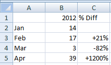
How to use cell values for excel chart labels - How to We want to chart the sales values and use the change values for data labels. Use Cell Values for Chart Data Labels. Select range A1:B6 and click Insert > Insert Column or Bar Chart > Clustered Column. The column chart will appear. We want to add data labels to show the change in value for each product compared to last month. Select the chart ...
Add Total Label On Stacked Bar Chart In Excel - YouTube
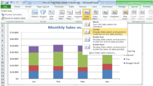
How to Add Data Labels in Excel - Excelchat | Excelchat After inserting a chart in Excel 2010 and earlier versions we need to do the followings to add data labels to the chart; Click inside the chart area to display the Chart Tools. Figure 2. Chart Tools Click on Layout tab of the Chart Tools. In Labels group, click on Data Labels and select the position to add labels to the chart. Figure 3.

How to Make Charts and Graphs in Excel | Smartsheet
How to create Custom Data Labels in Excel Charts Create the chart as usual Add default data labels Click on each unwanted label (using slow double click) and delete it Select each item where you want the custom label one at a time Press F2 to move focus to the Formula editing box Type the equal to sign Now click on the cell which contains the appropriate label Press ENTER That's it.

Chart Data Labels in PowerPoint 2011 for Mac
How to add text labels on Excel scatter chart axis - Data Cornering By default, you can not add text labels on Excel scatter chart axis, but here is a workaround that allows you to do that. You can change Excel scatter chart horizontal or vertical axis labels using a dummy series. Here is how to do that in a few simple steps. Here is the data that I would like to display in the Excel scatter chart. In addition ...
How to Show Percentages in Stacked Bar and Column Charts in Excel
How to add text labels on Excel scatter chart axis - Data Cornering Add dummy series to the scatter plot and add data labels. 4. Select recently added labels and press Ctrl + 1 to edit them. Add custom data labels from the column "X axis labels". Use "Values from Cells" like in this other post and remove values related to the actual dummy series. Change the label position below data points.
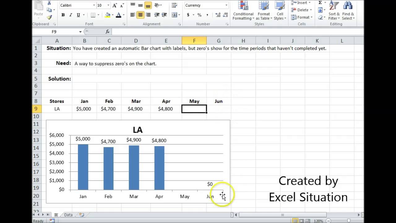
Excel Bar Chart Suppress Zeros - YouTube
Adding Data Labels To An Excel Chart | MyExcelOnline In our example below, I add a Data Label to a column chart and then I format the data label using CTRL+1. I then select to custom format the numbers so it shows the values as thousands by adding a comma , after each zero and then showing the work k by adding "k" Example Custom Number Format: [$$-1004]#,##0 ,"k" ;- [$$-1004]#,##0 ,"k"

Creating Pie Chart and Adding/Formatting Data Labels (Excel) - YouTube
How to add data labels from different column in an Excel chart? Please do as follows: 1. Right click the data series in the chart, and select Add Data Labels > Add Data Labels from the context menu to add... 2. Right click the data series, and select Format Data Labels from the context menu. 3. In the Format Data Labels pane, under Label Options tab, check the ...
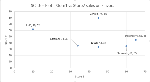
Add Custom Labels to x-y Scatter plot in Excel - DataScience Made Simple
Chart.ApplyDataLabels method (Excel) | Microsoft Docs The type of data label to apply. True to show the legend key next to the point. The default value is False. True if the object automatically generates appropriate text based on content. For the Chart and Series objects, True if the series has leader lines. Pass a Boolean value to enable or disable the series name for the data label.

30 How To Add Label To Excel Chart - Labels Database 2020

Charts in Excel - EASY Excel Tutorial

Part 2—Explore Biodiversity Using A Forest Inventory Growth (FIG) Dataset from Maine
How-to Add Custom Labels that Dynamically Change in Excel Charts - Excel Dashboard Templates

Create Custom Data Labels in Excel Charts - YouTube
Post a Comment for "41 excel chart add data labels"