41 excel chart custom data labels

How to create Custom Data Labels in Excel Charts Create the chart as usual Add default data labels Click on each unwanted label (using slow double click) and delete it Select each item where you want the custom label one at a time Press F2 to move focus to the Formula editing box Type the equal to sign Now click on the cell which contains the appropriate label Press ENTER That's it. Apply Custom Data Labels to Charted Points - Peltier Tech There are a number of ways to apply custom data labels to your chart: Manually Type Desired Text for Each Label Manually Link Each Label to Cell with Desired Text Use the Chart Labeler Program Use Values from Cells (Excel 2013 and later) Write Your Own VBA Routines Manually Type Desired Text for Each Label

Change the format of data labels in a chart To get there, after adding your data labels, select the data label to format, and then click Chart Elements > Data Labels > More Options. To go to the appropriate area, click one of the four icons ( Fill & Line, Effects, Size & Properties ( Layout & Properties in Outlook or Word), or Label Options) shown here.

Excel chart custom data labels

Excel Custom Chart Labels • My Online Training Hub While in the Format Axis dialog box go to the 'Line Colour' tab > select No Line Move the legend to the bottom: double click the legend > legend position > Bottom Get rid of the gridlines - just select them and press the Delete key. Add / Move Data Labels in Charts - Excel & Google Sheets Add and Move Data Labels in Google Sheets Double Click Chart Select Customize under Chart Editor Select Series 4. Check Data Labels 5. Select which Position to move the data labels in comparison to the bars. Final Graph with Google Sheets After moving the dataset to the center, you can see the final graph has the data labels where we want. » Excel Charts: Creating Custom Data Labels In this video I'll show you how to add data labels to a chart and then change the range that the data labels are linked to. If you are using Excel 2013 or above on Windows, there is a simple way to do this. However if you're using an earlier version or you're using Excel 2106 on the Mac, it's more of a manual process. The video covers both.

Excel chart custom data labels. Custom data labels in a chart - Get Digital Help Add data labels Press with right mouse button on on a column Press with left mouse button on "Add Data Labels" Double press with left mouse button on a data label Deselect Value Select Category name Press with left mouse button on Close Get the Excel file Custom-data-labels-in-a-chartv3.xlsx How to add or move data labels in Excel chart? - ExtendOffice In Excel 2013 or 2016. 1. Click the chart to show the Chart Elements button . 2. Then click the Chart Elements, and check Data Labels, then you can click the arrow to choose an option about the data labels in the sub menu. See screenshot: In Excel 2010 or 2007. 1. click on the chart to show the Layout tab in the Chart Tools group. See ... Excel charts: add title, customize chart axis, legend and data labels ... Click the Chart Elements button, and select the Data Labels option. For example, this is how we can add labels to one of the data series in our Excel chart: For specific chart types, such as pie chart, you can also choose the labels location. For this, click the arrow next to Data Labels, and choose the option you want. Add a DATA LABEL to ONE POINT on a chart in Excel All the data points will be highlighted. Click again on the single point that you want to add a data label to. Right-click and select ' Add data label '. This is the key step! Right-click again on the data point itself (not the label) and select ' Format data label '. You can now configure the label as required — select the content of ...

Create Custom Data Labels in Excel Charts - YouTube Video explains the procedure for labeling data points in a line chart with custom text. It shows how to create custom data labels in excel. Improve your X Y Scatter Chart with custom data labels Thank you for your Excel 2010 workaround for custom data labels in XY scatter charts. It basically works for me until I insert a new row in the worksheet associated with the chart. Doing so breaks the absolute references to data labels after the inserted row and Excel won't let me change the data labels to relative references. How to Customize Your Excel Pivot Chart Data Labels - dummies The Data Labels command on the Design tab's Add Chart Element menu in Excel allows you to label data markers with values from your pivot table. When you click the command button, Excel displays a menu with commands corresponding to locations for the data labels: None, Center, Left, Right, Above, and Below. How to add data labels from different column in an Excel chart? Right click the data series in the chart, and select Add Data Labels > Add Data Labels from the context menu to add data labels. 2. Click any data label to select all data labels, and then click the specified data label to select it only in the chart. 3.

Custom Chart Data Labels In Excel With Formulas Follow the steps below to create the custom data labels. Select the chart label you want to change. In the formula-bar hit = (equals), select the cell reference containing your chart label's data. In this case, the first label is in cell E2. Finally, repeat for all your chart laebls. Dynamically Label Excel Chart Series Lines • My Online ... Sep 26, 2017 · To modify the axis so the Year and Month labels are nested; right-click the chart > Select Data > Edit the Horizontal (category) Axis Labels > change the ‘Axis label range’ to include column A. Step 2: Clever Formula. The Label Series Data contains a formula that only returns the value for the last row of data. Excel Gantt Chart Tutorial + Free Template + Export to PPT Right-click the white chart space and click Select Data to bring up Excel's Select Data Source window. On the left side of Excel's Data Source window, you will see a table named Legend Entries (Series). Click on the Add button to bring up Excel's Edit Series window where you will begin adding the task data to your Gantt chart. Add or remove data labels in a chart - support.microsoft.com Click the data series or chart. To label one data point, after clicking the series, click that data point. In the upper right corner, next to the chart, click Add Chart Element > Data Labels. To change the location, click the arrow, and choose an option. If you want to show your data label inside a text bubble shape, click Data Callout.

Add Custom Labels to x-y Scatter plot in Excel - DataScience Made Simple

Custom Excel Chart Label Positions - My Online Training Hub A solution to this is to use custom Excel chart label positions assigned to a ghost series. For example, in the Actual vs Target chart below, only the Actual columns have labels and it doesn't matter whether they're aligned to the top or base of the column, they don't look great because many of them are partially covered by the target column:

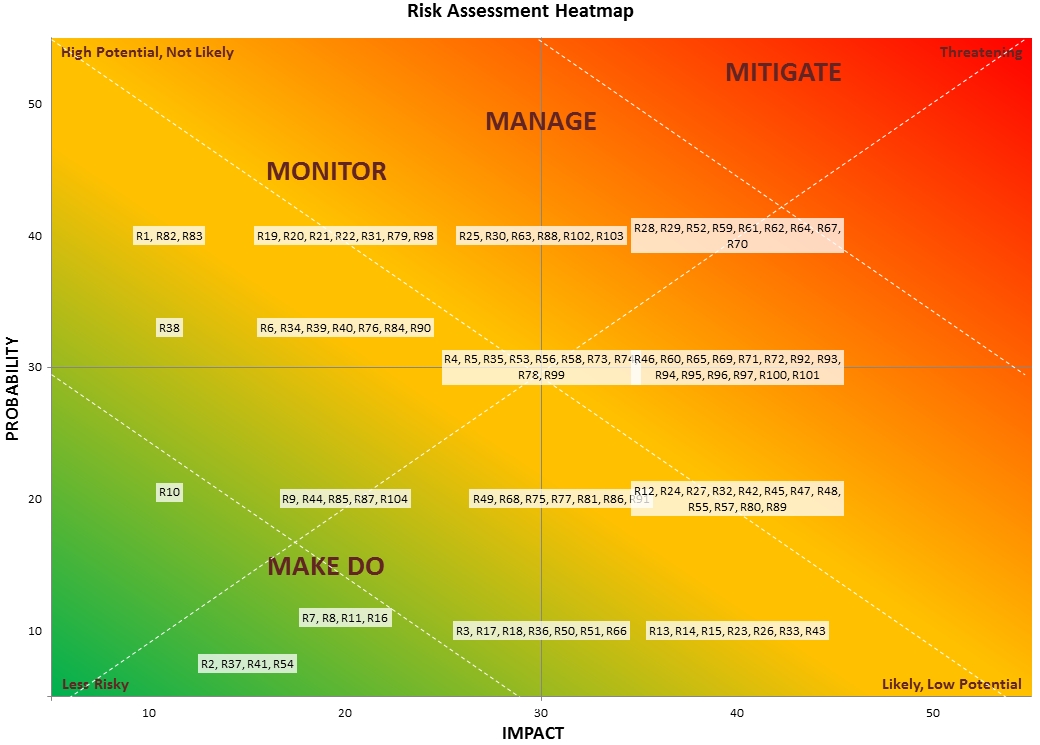
How to Create a Risk Heatmap in Excel - Part 2 - Risk Management Guru

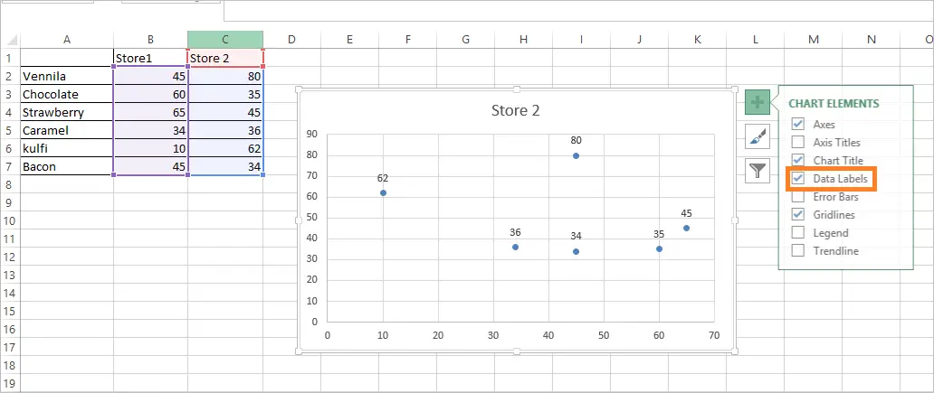
Add Custom Labels to x-y Scatter plot in Excel Step 1: Select the Data, INSERT -> Recommended Charts -> Scatter chart (3 rd chart will be scatter chart) Let the plotted scatter chart be. Step 2: Click the + symbol and add data labels by clicking it as shown below. Step 3: Now we need to add the flavor names to the label. Now right click on the label and click format data labels.

How to Customize Your Excel Pivot Chart Data Labels - dummies

Adding rich data labels to charts in Excel 2013 - Microsoft 365 Blog Putting a data label into a shape can add another type of visual emphasis. To add a data label in a shape, select the data point of interest, then right-click it to pull up the context menu. Click Add Data Label, then click Add Data Callout . The result is that your data label will appear in a graphical callout.

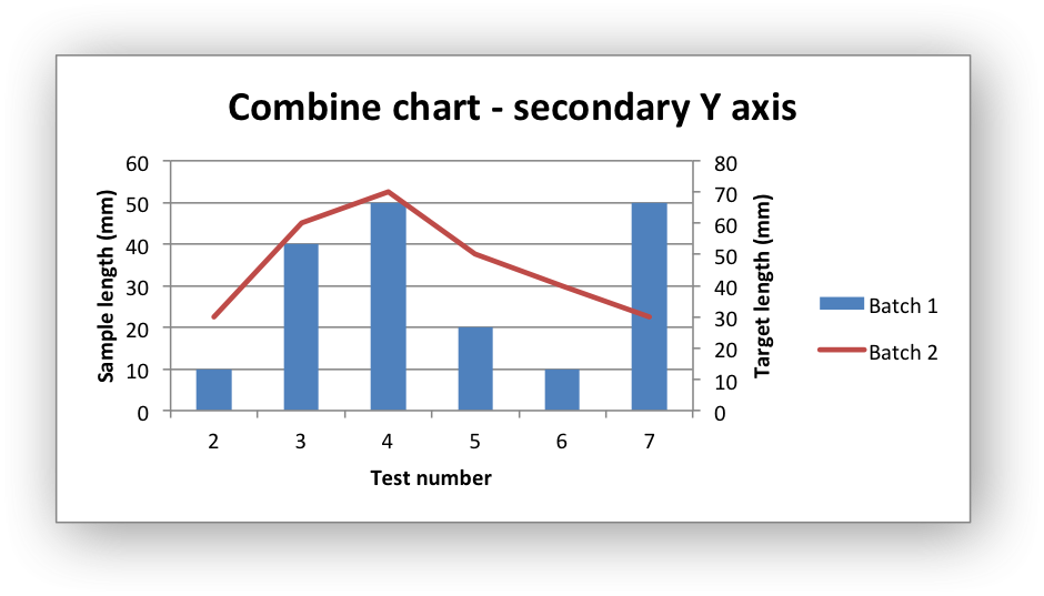
Example: Combined Chart — XlsxWriter Documentation

Xlsxwriter Excel Chart Custom Data Label Position At default the custom labels seem to bet set at right. I want them on top but I cant get this. The code is like that: chart.add_series ( .., 'data_labels': {'custom': my_custom_labels, 'position': 'above'}) But the changes wont appy to the chart. I also found i can set the default label position (label_position_default) in the chart object ...

Custom Data Labels with Colors and Symbols in Excel Charts – [How To] - KING OF EXCEL

How to Change Excel Chart Data Labels to Custom Values? You can change data labels and point them to different cells using this little trick. First add data labels to the chart (Layout Ribbon > Data Labels) Define the new data label values in a bunch of cells, like this: Now, click on any data label. This will select "all" data labels. Now click once again.

Custom Data Labels with Colors and Symbols in Excel Charts - [How To] - PakAccountants.com

Using the CONCAT function to create custom data labels for an Excel chart Use the chart skittle (the "+" sign to the right of the chart) to select Data Labels and select More Options to display the Data Labels task pane. Check the Value From Cells checkbox and select the cells containing the custom labels, cells C5 to C16 in this example.

How to Change Excel Chart Data Labels to Custom Values?

DataLabels object (Excel) | Microsoft Docs The following example sets the number format for data labels on series one on chart sheet one. With Charts(1).SeriesCollection(1) .HasDataLabels = True .DataLabels.NumberFormat = "##.##" End With Use DataLabels (index), where index is the data-label index number, to return a single DataLabel object. The following example sets the number format ...

How to Make Charts and Graphs in Excel | Smartsheet

Use custom formats in an Excel chart's axis and data labels Right-click the Axis area and choose Format Axis from the context menu. If you don't see Format Axis, right-click another spot. Choose Number in the left pane. (In Excel 2003, click the Number ...

Add Custom Labels to x-y Scatter plot in Excel - DataScience Made Simple

Custom Data Labels with Colors and Symbols in Excel Charts - [How To] The basic idea behind custom label is to connect each data label to certain cell in the Excel worksheet and so whatever goes in that cell will appear on the chart as data label. So once a data label is connected to a cell, we apply custom number formatting on the cell and the results will show up on chart also.

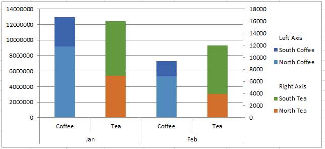
How-to Group and Categorize Excel Chart Legend Entries - Excel Dashboard Templates

How To Use Dynamic Data Labels To Create Interactive Excel Charts To create a column chart with dynamic data labels, you need to follow these given steps. Select the data & Create a Combo Chart. Now select the column chart for revenue data and a line chart with marker for data labels. Add Data Labels to the Line Chart With Marker. After then remove the Line Color and Marker Color.

How-to Use Data Labels from a Range in an Excel Chart - Excel Dashboard Templates

Excel Charts: Creating Custom Data Labels - YouTube Excel Charts: Creating Custom Data Labels 84,148 views Jun 26, 2016 191 Dislike Share Save Mike Thomas 4.48K subscribers Subscribe In this video I'll show you how to add data labels to a chart in...

30 How To Add Label To Excel Chart - Labels Database 2020

Modify Excel Chart Data Range | CustomGuide The new data needs to be in cells adjacent to the existing chart data. Rename a Data Series. Charts are not completely tied to the source data. You can change the name and values of a data series without changing the data in the worksheet. Select the chart; Click the Design tab. Click the Select Data button.

10+ ways to make Excel Variance Reports and Charts - How To - PakAccountants.com

Add Data Points to Existing Chart – Excel & Google Sheets Similar to Excel, create a line graph based on the first two columns (Months & Items Sold) Right click on graph; Select Data Range . 3. Select Add Series. 4. Click box for Select a Data Range. 5. Highlight new column and click OK. Final Graph with Single Data Point

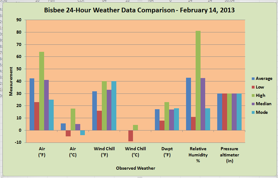
WeatherData

» Excel Charts: Creating Custom Data Labels In this video I'll show you how to add data labels to a chart and then change the range that the data labels are linked to. If you are using Excel 2013 or above on Windows, there is a simple way to do this. However if you're using an earlier version or you're using Excel 2106 on the Mac, it's more of a manual process. The video covers both.

35 How To Label In Excel - Labels Database 2020

Add / Move Data Labels in Charts - Excel & Google Sheets Add and Move Data Labels in Google Sheets Double Click Chart Select Customize under Chart Editor Select Series 4. Check Data Labels 5. Select which Position to move the data labels in comparison to the bars. Final Graph with Google Sheets After moving the dataset to the center, you can see the final graph has the data labels where we want.

Share :